Understanding Diffusion Models

Diffusion models were first introduced in the seminal work by [Sohl-Dickstein et al. (2015)](https://arxiv.org/abs/1503.03585). The core idea involves reversing a Markov chain-based forward diffusion process, which gradually degrades the structure of the data $\mathbf{z}_0$ from the real data distribution $q(\mathbf{z}_0)$, by adding noise over a sufficient number of steps. When this noise is Gaussian, as is commonly assumed in practice, the cumulative effect transforms the data distribution towards a standard normal distribution $\mathcal{N}(0, I)$ as the forward process progresses. We can then sample from this distribution and use a learned reverse process to generate new samples that match the real data distribution. Specifically, as illustrated in Figure 1, we define the forward diffusion process $q$ that gradually applies Gaussian noise to the data distribution $\mathbf{z}_0 \sim q(\mathbf{z}_0)$ with a variance schedule $\beta_t \in (0, 1)$ as follows: $$ q(\mathbf{z}_{1:T} \vert \mathbf{z}_0) := \prod_{t=1}^T q(\mathbf{z}_t \vert \mathbf{z}_{t-1}) \tag{1} $$ $$ q(\mathbf{z}_t \vert \mathbf{z}_{t-1}) := \mathcal{N}(\mathbf{z}_t; \sqrt{1 - \beta_t} \mathbf{z}_{t-1}, \beta_t \mathbf{I}) \tag{2} $$
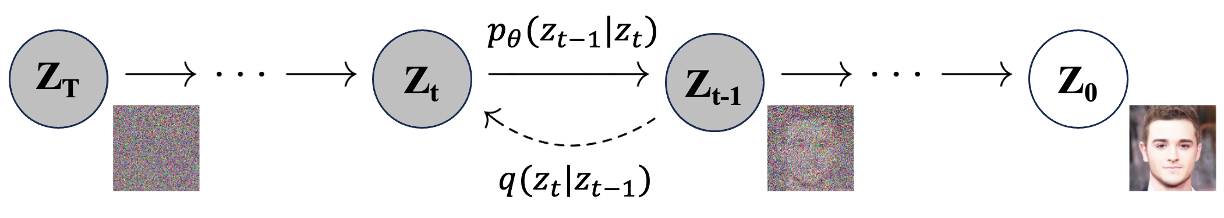*Figure 1: Illustration of the forward and reverse diffusion process. Figure adapted from [Ho et al. (2020)](https://arxiv.org/abs/2006.11239).* Here, $t$ and $T$ refer to the current and total timesteps, respectively. With a sufficiently large $T$ and a properly defined variance schedule $\beta$, the final $\mathbf{z}_T$ will approximate an isotropic Gaussian distribution, where variances are equal in all directions. We can then reverse the forward diffusion process by starting from $\mathbf{z}_T \sim \mathcal{N}(0, I)$ and gradually obtain a sample $\mathbf{z}_0$ that resembles the real data distribution $q(\mathbf{z}_0)$, defined as follows: $$ p_{\theta}(\mathbf{z}_{0:T}) := p(\mathbf{z}_T) \prod_{t=1}^{T} p_{\theta}(\mathbf{z}_{t-1} \vert \mathbf{z}_{t}) \tag{3} $$ $$ p_{\theta}(\mathbf{z}_{t-1} \vert \mathbf{z}_{t}) := \mathcal{N}(\mathbf{z}_{t-1}; \mu_{\theta}(\mathbf{z}_{t}, t), \Sigma_{\theta}(\mathbf{z}_{t}, t)) \tag{4} $$ Where all $\mathbf{z}_t$ for $t \in \{0, 1, \ldots, T \}$ share the same dimensionality, $p_{\theta}(\mathbf{z}_{t-1} \vert \mathbf{z}_{t})$ is practically a neural network learned to approximate the actual reverse distribution $q(\mathbf{z}_{t-1} \vert \mathbf{z}_{t})$, as it depends on the entire dataset which is not easily accessible. The term $p_{\theta}(\mathbf{z}_{0:T})$ denotes the entire learned reverse process. An interesting property of the forward process is the existence of a closed-form sampling solution for $\mathbf{z}_t$ at an arbitrary $t \in [0, T]$ using the reparameterization trick. By defining $\alpha_t := 1 - \beta_t$ and $\bar{\alpha}_t := \prod_{i=1}^{t} \alpha_i$, given Equation 2, and recall that $\mathcal{N}(z; \mu, \sigma^2\mathbf{I})$ is equivalent to $z = \mu + \sigma \epsilon$ where $\epsilon \sim \mathcal{N}(0, 1)$, we obtain: $$ \begin{align} \mathbf{z}_t &= \sqrt{1 - \beta_t} \mathbf{z}_{t-1} + \sqrt{\beta_t} \boldsymbol{\epsilon} \tag{5} \\ &= \sqrt{\alpha_t} \mathbf{z}_{t-1} + \sqrt{1 - \alpha_t} \boldsymbol{\epsilon} \tag{6} \\ &= \sqrt{\alpha_t \alpha_{t-1}} \mathbf{z}_{t-2} + \sqrt{1 - \alpha_t \alpha_{t-1}} \boldsymbol{\epsilon} \tag{7} \\ &= \sqrt{\alpha_t \alpha_{t-1} \alpha_{t-2}} \mathbf{z}_{t-3} + \sqrt{1 - \alpha_t \alpha_{t-1} \alpha_{t-2}} \boldsymbol{\epsilon} \tag{8} \\ &\quad \vdots \notag \\ &= \sqrt{\alpha_t \alpha_{t-1} \ldots \alpha_1 \alpha_0} \mathbf{z}_0 + \sqrt{1 - \alpha_t \alpha_{t-1} \ldots \alpha_1 \alpha_0} \boldsymbol{\epsilon} \tag{9} \\ &= \sqrt{\bar{\alpha}_t} \mathbf{z}_0 + \sqrt{1 - \bar{\alpha}_t} \boldsymbol{\epsilon} \tag{10} \end{align} $$ Which leads to: $$ q(\mathbf{z}_t \vert \mathbf{z}_0) = \mathcal{N}(\mathbf{z}_t; \sqrt{\bar{\alpha}_t} \mathbf{z}_0, (1 - \bar{\alpha}_t) \mathbf{I}) \tag{11} $$ Recall that combining two Gaussian distributions with different variances, $\mathcal{N}(z; \mu, \sigma_1^2\mathbf{I})$ and $\mathcal{N}(z; \mu, \sigma_2^2\mathbf{I})$, results in $\mathcal{N}(z; \mu, (\sigma_1^2+\sigma_2^2)\mathbf{I})$. Thus, in the case of Equation 7, for transitioning from $t$ to $t-1$, the variance becomes $\sqrt{(1 - \alpha_t) + \alpha_t (1-\alpha_{t-1})} = \sqrt{1 - \alpha_t\alpha_{t-1}}$, with subsequent derivations following the same intuition. The goal is to learn a network $p_\theta$ that can approximate the actual reverse process. We start by looking at the objective that we want to minimize: the negative log-likelihood, $- \log p_\theta(\mathbf{z}_0)$, which involves maximizing the likelihood of the real data. However, directly optimizing this objective is practically infeasible due to its dependence on the entire sequence of previous steps. As a solution ([Sohl-Dickstein et al. (2015)](https://arxiv.org/abs/1503.03585)), we can derive an variational lower bound (vlb) on the data log-likelihood to achieve the same optimization effect: $$ \begin{align} - \log p_\theta(\mathbf{z}_0) &\leq - \log p_\theta(\mathbf{z}_0) + D_\text{KL}(q(\mathbf{z}_{1:T} \vert \mathbf{z}_0) \Vert p_\theta(\mathbf{z}_{1:T} \vert \mathbf{z}_0)) \tag{12} \\ &= -\log p_\theta(\mathbf{z}_0) + \mathbb{E}_q \left[ \log \frac{q(\mathbf{z}_{1:T} \vert \mathbf{z}_0)}{p_\theta(\mathbf{z}_{1:T} \vert \mathbf{z}_0)} \right] \tag{13} \\ &= -\log p_\theta(\mathbf{z}_0) + \mathbb{E}_q \left[ \log \frac{q(\mathbf{z}_{1:T} \vert \mathbf{z}_0)}{p_\theta(\mathbf{z}_{0}, \mathbf{z}_{1:T}) / p_\theta(\mathbf{z}_{0})} \right], \quad \text{using Bayes' rule} \tag{14} \\ &= -\log p_\theta(\mathbf{z}_0) + \mathbb{E}_q \left[ \log \frac{q(\mathbf{z}_{1:T} \vert \mathbf{z}_0)}{p_\theta(\mathbf{z}_{0:T}) / p_\theta(\mathbf{z}_0)} \right] \tag{15} \\ &= -\log p_\theta(\mathbf{z}_0) + \mathbb{E}_q \left[ \log \frac{q(\mathbf{z}_{1:T} \vert \mathbf{z}_0)}{p_\theta(\mathbf{z}_{0:T})} + \log p_\theta(\mathbf{z}_0) \right] \tag{16} \\ &= \mathbb{E}_q \left[ \log \frac{q(\mathbf{z}_{1:T} \vert \mathbf{z}_0)}{p_\theta(\mathbf{z}_{0:T})} \right] := L_{vlb} \tag{17} \end{align} $$ Note that the numerator and denominator of $L_{vlb}$ refer to the forward process and the learned reverse process, respectively. Therefore, we can derive the following expressions ([Sohl-Dickstein et al. (2015)](https://arxiv.org/abs/1503.03585), [Ho et al. (2020)](https://arxiv.org/abs/2006.11239)): $$ \begin{align} L_\text{vlb} &= \mathbb{E}_{q} \Bigg[ \log\frac{q(\mathbf{z}_{1:T}\vert\mathbf{z}_0)}{p_\theta(\mathbf{z}_{0:T})} \Bigg] \tag{18} \\ &= \mathbb{E}_q \Bigg[ \log\frac{\prod_{t=1}^T q(\mathbf{z}_t\vert\mathbf{z}_{t-1})}{ p(\mathbf{z}_T) \prod_{t=1}^T p_\theta(\mathbf{z}_{t-1} \vert\mathbf{z}_t) } \Bigg] \tag{19} \\ &= \mathbb{E}_q \Bigg[ -\log p(\mathbf{z}_T) + \sum_{t=1}^T \log \frac{q(\mathbf{z}_t\vert\mathbf{z}_{t-1})}{p_\theta(\mathbf{z}_{t-1} \vert\mathbf{z}_t)} \Bigg], \quad \text{using Logarithmic rules} \tag{20} \\ &= \mathbb{E}_q \Bigg[ -\log p(\mathbf{z}_T) + \sum_{t=2}^T \log \frac{q(\mathbf{z}_t\vert\mathbf{z}_{t-1})}{p_\theta(\mathbf{z}_{t-1} \vert\mathbf{z}_t)} + \log\frac{q(\mathbf{z}_1 \vert \mathbf{z}_0)}{p_\theta(\mathbf{z}_0 \vert \mathbf{z}_1)} \Bigg] \tag{21} \end{align} $$ Here, given the intrinsically high variance in the intermediate samples that introduces intractability in modeling the reverse process, we can condition on $\mathbf{z}_0$ due to its accessibility and feasibility to reduce the variance and make it tractable: $$ \begin{align} L_\text{vlb} &= \mathbb{E}_q \Bigg[ -\log p(\mathbf{z}_T) + \sum_{t=2}^T \log \frac{q(\mathbf{z}_t\vert\mathbf{z}_{t-1})}{p_\theta(\mathbf{z}_{t-1} \vert\mathbf{z}_t)} + \log\frac{q(\mathbf{z}_1 \vert \mathbf{z}_0)}{p_\theta(\mathbf{z}_0 \vert \mathbf{z}_1)} \Bigg] \tag{22} \\ &= \mathbb{E}_q \Bigg[ -\log p(\mathbf{z}_T) + \sum_{t=2}^T \log \frac{q(\mathbf{z}_{t-1}\vert\mathbf{z}_{t}) q(\mathbf{z}_t)}{p_\theta(\mathbf{z}_{t-1} \vert\mathbf{z}_t) q(\mathbf{z}_{t-1})} + \log\frac{q(\mathbf{z}_1 \vert \mathbf{z}_0)}{p_\theta(\mathbf{z}_0 \vert \mathbf{z}_1)} \Bigg], \quad \text{using Bayes' rule} \tag{23} \\ &= \mathbb{E}_q \Bigg[ -\log p(\mathbf{z}_T) + \sum_{t=2}^T \log \Bigg( \frac{q(\mathbf{z}_{t-1} \vert \mathbf{z}_t, \mathbf{z}_0)}{p_\theta(\mathbf{z}_{t-1} \vert\mathbf{z}_t)} \cdot \frac{q(\mathbf{z}_t \vert \mathbf{z}_0)}{q(\mathbf{z}_{t-1}\vert\mathbf{z}_0)} \Bigg) + \log \frac{q(\mathbf{z}_1 \vert \mathbf{z}_0)}{p_\theta(\mathbf{z}_0 \vert \mathbf{z}_1)} \Bigg] \tag{24} \\ &= \mathbb{E}_q \Bigg[ -\log p(\mathbf{z}_T) + \sum_{t=2}^T \log \frac{q(\mathbf{z}_{t-1} \vert \mathbf{z}_t, \mathbf{z}_0)}{p_\theta(\mathbf{z}_{t-1} \vert\mathbf{z}_t)} + \sum_{t=2}^T \log \frac{q(\mathbf{z}_t \vert \mathbf{z}_0)}{q(\mathbf{z}_{t-1} \vert \mathbf{z}_0)} + \log\frac{q(\mathbf{z}_1 \vert \mathbf{z}_0)}{p_\theta(\mathbf{z}_0 \vert \mathbf{z}_1)} \Bigg] \tag{25} \end{align} $$ Here, since the term $\sum_{t=2}^T \log \frac{q(\mathbf{z}_t \vert \mathbf{z}_0)}{q(\mathbf{z}_{t-1} \vert \mathbf{z}_0)}$ can be unrolled as: $$ \sum_{t=2}^T \log \frac{q(\mathbf{z}_t \vert \mathbf{z}_0)}{q(\mathbf{z}_{t-1} \vert \mathbf{z}_0)} = \log \left( \frac{q(z_2 \vert z_0) q(z_3 \vert z_0) q(z_4 \vert z_0) \cdots q(z_T \vert z_0)}{q(z_1 \vert z_0) q(z_2 \vert z_0) q(z_3 \vert z_0) \cdots q(z_{T-1} \vert z_0)} \right) \tag{26} $$ Where the intermediate terms cancel out, resulting in $\log \frac{q(\mathbf{z}_T \vert \mathbf{z}_0)}{q(\mathbf{z}_{1} \vert \mathbf{z}_0)}$, we can then continue the derivation as follows: $$ \begin{align} L_\text{vlb} &= \mathbb{E}_q \Bigg[ -\log p(\mathbf{z}_T) + \sum_{t=2}^T \log \frac{q(\mathbf{z}_{t-1} \vert \mathbf{z}_t, \mathbf{z}_0)}{p_\theta(\mathbf{z}_{t-1} \vert\mathbf{z}_t)} + \sum_{t=2}^T \log \frac{q(\mathbf{z}_t \vert \mathbf{z}_0)}{q(\mathbf{z}_{t-1} \vert \mathbf{z}_0)} + \log\frac{q(\mathbf{z}_1 \vert \mathbf{z}_0)}{p_\theta(\mathbf{z}_0 \vert \mathbf{z}_1)} \Bigg] \tag{27} \\ &= \mathbb{E}_q \Bigg[ -\log p(\mathbf{z}_T) + \sum_{t=2}^T \log \frac{q(\mathbf{z}_{t-1} \vert \mathbf{z}_t, \mathbf{z}_0)}{p_\theta(\mathbf{z}_{t-1} \vert\mathbf{z}_t)} + \log\frac{q(\mathbf{z}_T \vert \mathbf{z}_0)}{q(\mathbf{z}_1 \vert \mathbf{z}_0)} + \log \frac{q(\mathbf{z}_1 \vert \mathbf{z}_0)}{p_\theta(\mathbf{z}_0 \vert \mathbf{z}_1)} \Bigg] \tag{28} \\ &= \mathbb{E}_q \Bigg[ \log\frac{q(\mathbf{z}_T \vert \mathbf{z}_0)}{p(\mathbf{z}_T)} + \sum_{t=2}^T \log \frac{q(\mathbf{z}_{t-1} \vert \mathbf{z}_t, \mathbf{z}_0)}{p_\theta(\mathbf{z}_{t-1} \vert\mathbf{z}_t)} - \log p_\theta(\mathbf{z}_0 \vert \mathbf{z}_1) \Bigg], \quad \text{using Logarithmic rules} \tag{29} \\ &= \mathbb{E}_q \Bigg[ \underbrace{D_\text{KL}(q(\mathbf{z}_T \vert \mathbf{z}_0) \parallel p(\mathbf{z}_T))}_{L_T} + \sum_{t=2}^T \underbrace{D_\text{KL}(q(\mathbf{z}_{t-1} \vert \mathbf{z}_t, \mathbf{z}_0) \parallel p_\theta(\mathbf{z}_{t-1} \vert\mathbf{z}_t))}_{L_{t-1}} \underbrace{- \log p_\theta(\mathbf{z}_0 \vert \mathbf{z}_1)}_{L_0} \Bigg] \tag{30} \end{align} $$ Recall that in Equation 2, the forward process requires a variance term $\beta_t$, which can either be learned through reparameterization ([Kingma and Welling (2013)](https://arxiv.org/abs/1312.6114)) or treated as hyperparameters fixed as time-dependent constants, both retaining the same functional form ([Sohl-Dickstein et al. (2015)](https://arxiv.org/abs/1503.03585)). The subsequent groundbreaking work by [Ho et al. (2020)](https://arxiv.org/abs/2006.11239) adopts the latter approach. Specifically, $\beta_t$ is set according to a linearly increasing schedule within a specific range based on the timesteps, although subsequent work ([Nichol and Dhariwal (2021)](https://arxiv.org/abs/2102.09672)) has proposed other scheduling schemes. Given that we have fixed the forward process variances $\beta_t$, in Equation 30, since $\mathbf{z}_T$ is Gaussian noise sampled from $\mathcal{N}(0, I)$ and $q$ has no learnable parameters, while $p(\mathbf{z}_T)$ converges to the normal distribution $\mathcal{N}(0, I)$ given a sufficiently large $T$. Therefore, the $L_T$ term is constant and typically small, allowing it to be ignored, and we only need to focus on minimizing the $L_{t-1}$ and $L_0$ terms. Recall that conditioning on $\mathbf{z}_0$ in Equation 24 makes the reverse posterior tractable, let: $$ q(\mathbf{z}_{t-1} \vert \mathbf{z}_t, \mathbf{z}_0) = \mathcal{N}(\mathbf{z}_{t-1}; {\tilde{\mu}}(\mathbf{z}_t, \mathbf{z}_0), {\tilde{\beta}_t} \mathbf{I}) \tag{31} $$ Also recall that the Gaussian density function $\mathcal{N}(z; \mu, \sigma^2)$ can be written as: $$ \begin{align} \mathcal{N}(z; \mu, \sigma^2) &= \frac{1}{\sqrt{2 \pi \sigma^2}} \exp\left(-\frac{(z - \mu)^2}{2\sigma^2}\right) \tag{32} \\ &\propto \exp\left(-\frac{(z - \mu)^2}{2\sigma^2}\right) \quad = \exp\left(-\frac{(z^2 - 2z\mu + \mu^2)}{2\sigma^2}\right) \tag{33} \end{align} $$ We can then derive the followings: $$ \begin{align} q(\mathbf{z}_{t-1} \vert \mathbf{z}_t, \mathbf{z}_0) &= q(\mathbf{z}_t \vert \mathbf{z}_{t-1}, \mathbf{z}_0) \frac{ q(\mathbf{z}_{t-1} \vert \mathbf{z}_0) }{ q(\mathbf{z}_t \vert \mathbf{z}_0) }, \quad \text{using Bayes' rule} \tag{34} \\ &\propto \exp \left( -\frac{1}{2} \left( \frac{(\mathbf{z}_t - \sqrt{\alpha_t} \mathbf{z}_{t-1})^2}{\beta_t} \right. \right. \notag \\ &\qquad \left. \left. + \frac{(\mathbf{z}_{t-1} - \sqrt{\bar{\alpha}_{t-1}} \mathbf{z}_0)^2}{1-\bar{\alpha}_{t-1}} - \frac{(\mathbf{z}_t - \sqrt{\bar{\alpha}_t} \mathbf{z}_0)^2}{1-\bar{\alpha}_t} \right) \right) \tag{35} \\ &= \exp \left( -\frac{1}{2} \left( \frac{\mathbf{z}_t^2 - 2\sqrt{\alpha_t} \mathbf{z}_t \mathbf{z}_{t-1} + \alpha_t \mathbf{z}_{t-1}^2}{\beta_t} \right. \right. \notag \\ &\qquad \left. \left. + \frac{\mathbf{z}_{t-1}^2 - 2 \sqrt{\bar{\alpha}_{t-1}} \mathbf{z}_0 \mathbf{z}_{t-1} + \bar{\alpha}_{t-1} \mathbf{z}_0^2}{1-\bar{\alpha}_{t-1}} - \frac{(\mathbf{z}_t - \sqrt{\bar{\alpha}_t} \mathbf{z}_0)^2}{1-\bar{\alpha}_t} \right) \right) \tag{36} \\ &= \exp \left( -\frac{1}{2} \left( \left( \frac{\alpha_t}{\beta_t} + \frac{1}{1 - \bar{\alpha}_{t-1}} \right) \mathbf{z}_{t-1}^2 \right. \right. \notag \\ &\qquad \left. \left. - \left( \frac{2\sqrt{\alpha_t}}{\beta_t} \mathbf{z}_t + \frac{2\sqrt{\bar{\alpha}_{t-1}}}{1 - \bar{\alpha}_{t-1}} \mathbf{z}_0 \right) \mathbf{z}_{t-1} + \Lambda(\mathbf{z}_t, \mathbf{z}_0) \right) \right) \tag{37} \end{align} $$ Where the function $\Lambda(\mathbf{z}_t, \mathbf{z}_0)$ is irrelevant of $\mathbf{z}_{t-1}$, and hence is treated as a constant being ignored. By identifying the coefficients in Equation 37 as the form of: $$ -\frac{1}{2} \left( A z_{t-1}^2 - 2 B z_{t-1} + \Lambda \right) \tag{38} $$ With reference to Equation 31, we have: $$ \begin{align} \tilde{\beta}_t &= \frac{1}{A} = (\frac{\alpha_t}{\beta_t} + \frac{1}{1 - \bar{\alpha}_{t-1}})^{-1} = \frac{\beta_t (1 - \bar{\alpha}_{t-1})}{\alpha_t - \bar{\alpha}_t + \beta_t} = {\frac{1 - \bar{\alpha}_{t-1}}{1 - \bar{\alpha}_t} \cdot \beta_t} \tag{39} \\ \tilde{\mu}_t (\mathbf{z}_t, \mathbf{z}_0) &= \tilde{\beta}_tB = \Big(\frac{\sqrt{\alpha_t}}{\beta_t} \mathbf{z}_t + \frac{\sqrt{\bar{\alpha}_{t-1}}}{1 - \bar{\alpha}_{t-1}} \mathbf{z}_0\Big)\Big(\frac{\alpha_t}{\beta_t} + \frac{1}{1 - \bar{\alpha}_{t-1}}\Big)^{-1} \tag{40} \\ &= \left( \frac{\sqrt{\alpha_t}}{\beta_t} \mathbf{z}_t + \frac{\sqrt{\bar{\alpha}_{t-1}}}{1 - \bar{\alpha}_{t-1}} \mathbf{z}_0 \right) \Big({\frac{1 - \bar{\alpha}_{t-1}}{1 - \bar{\alpha}_t} \cdot \beta_t}\Big) \tag{41} \\ &= \frac{\sqrt{\alpha_t} (1 - \bar{\alpha}_{t-1})}{1 - \bar{\alpha}_t} \mathbf{z}_t + \frac{\sqrt{\bar{\alpha}_{t-1}} \beta_t}{1 - \bar{\alpha}_t} \mathbf{z}_0 \tag{42} \end{align} $$ Recall Equation 10, which allows us to directly sample $\mathbf{z}_t$ from $\mathbf{z}_0$ at any arbitrary $t$. Similarly, we can perform the reverse to obtain $\mathbf{z}_0$ directly from $\mathbf{z}_t$ at any arbitrary $t$, as follows: $$ \mathbf{z}_0 = \frac{\mathbf{z}_t - \sqrt{1 - \bar{\alpha}_t}\boldsymbol{\epsilon}}{\sqrt{\bar{\alpha}_t}} \tag{43} $$ Plugging into $\tilde{\mu}_t (\mathbf{z}_t, \mathbf{z}_0)$ in Equation 42, we can further simplify to: $$ \begin{align} \tilde{\mu}_t &= \frac{\sqrt{\alpha_t}(1 - \bar{\alpha}_{t-1})}{1 - \bar{\alpha}_t} \mathbf{z}_t + \Big(\frac{\sqrt{\bar{\alpha}_{t-1}}\beta_t}{1 - \bar{\alpha}_t}\Big) \Big(\frac{\mathbf{z}_t - \sqrt{1 - \bar{\alpha}_t}\boldsymbol{\epsilon}}{\sqrt{\bar{\alpha}_t}}\Big) \tag{44} \\ &= {\frac{1}{\sqrt{\alpha_t}} \Big( \mathbf{z}_t - \frac{1 - \alpha_t}{\sqrt{1 - \bar{\alpha}_t}} \boldsymbol{\epsilon} \Big)} \tag{45} \end{align} $$ Revisiting the reverse posterior in Equation (4), following the configuration as ([Ho et al. (2020)](https://arxiv.org/abs/2006.11239)), the reverse process variance $\boldsymbol{\Sigma}_\theta(\mathbf{z}_t, t) = \sigma^2_t \mathbf{I}$ is also set to be untrained time-dependent constants. Here, $\sigma^2_t$ is either $\beta_t$ or $\tilde{\beta}_t = \frac{1 - \bar{\alpha}_{t-1}}{1 - \bar{\alpha}_t} \cdot \beta_t$, both of which are claimed to yield similar empirical results. It is noteworthy that subsequent work ([Nichol and Dhariwal (2021)](https://arxiv.org/abs/2102.09672)) has proposed learning the variance $\boldsymbol{\Sigma}_\theta(\mathbf{z}_t, t)$ as an interpolation between $\beta_t$ and $\tilde{\beta}_t$, providing an alternative scheme. Returning to Equation (30), where we aim to minimize the $L_{t-1}$ term, given Equation (4) and Equation (31), recall that the $\beta_t$ term, which their variances depend on, is fixed to constants. This leaves only the mean $\mu_{\theta}(\mathbf{z}_{t}, t)$ to match. We can then parameterize $L_{t-1}$ as follows: $$ L_{t-1} = \mathbb{E}_{\mathbf{z}_0, \epsilon} \Bigg[ \frac{1}{2\sigma_t^2} \left\Vert \tilde{\mu}_t (\mathbf{z}_t, \mathbf{z}_0) - \mu_\theta (\mathbf{z}_t, t) \right\Vert^2 \Bigg] \tag{46} $$ Recall Equation (45), which we want the trained $\mu_{\theta}(\mathbf{z}_{t}, t)$ to match given $\mathbf{z}_t$. Since $\mathbf{z}_t$ is available as input during training, we can instead choose to fit the model on the noise, as derived below: $$ \begin{align} L_{t-1} &= \mathbb{E}_{\mathbf{z}_0, \epsilon} \Bigg[ \frac{1}{2\sigma_t^2} \left\Vert \tilde{\mu}_t (\mathbf{z}_t, \mathbf{z}_0) - \mu_\theta (\mathbf{z}_t, t) \right\Vert^2 \Bigg] \tag{47} \\ &= \mathbb{E}_{\mathbf{z}_0, \epsilon} \Bigg[ \frac{1}{2\sigma_t^2} \left\Vert {\frac{1}{\sqrt{\alpha_t}} \Big( \mathbf{z}_t - \frac{1 - \alpha_t}{\sqrt{1 - \bar{\alpha}_t}} \boldsymbol{\epsilon} \Big)} - {\frac{1}{\sqrt{\alpha_t}} \Big( \mathbf{z}_t - \frac{1 - \alpha_t}{\sqrt{1 - \bar{\alpha}_t}} \boldsymbol{\epsilon}_\theta(\mathbf{z}_t, t) \Big)} \right\Vert^2 \Bigg] \tag{48} \\ &= \mathbb{E}_{\mathbf{z}_0, \epsilon} \Bigg[ \frac{(1 - \alpha_t)^2}{2\sigma_t^2 \alpha_t (1 - \bar{\alpha}_t) } \left\Vert \boldsymbol{\epsilon} - \boldsymbol{\epsilon}_\theta (\mathbf{z}_t, t) \right\Vert^2 \Bigg] \tag{49} \\ &= \mathbb{E}_{\mathbf{z}_0, \epsilon} \Bigg[ \frac{(1 - \alpha_t)^2}{2\sigma_t^2 \alpha_t (1 - \bar{\alpha}_t) } \left\Vert \boldsymbol{\epsilon} - \boldsymbol{\epsilon}_\theta (\mathbf{z}_t, t) \right\Vert^2 \Bigg] \tag{50} \\ &= \mathbb{E}_{\mathbf{z}_0, \epsilon} \Bigg[ \frac{(1 - \alpha_t)^2}{2\sigma_t^2 \alpha_t (1 - \bar{\alpha}_t) } \left\Vert \boldsymbol{\epsilon} - \boldsymbol{\epsilon}_\theta (\sqrt{\bar{\alpha}_t} \mathbf{z}_0 + \sqrt{1 - \bar{\alpha}_t} \boldsymbol{\epsilon}, t) \right\Vert^2 \Bigg] \tag{51} \end{align} $$ Here, $\epsilon_\theta$ refers to the model predicting the noise given $z_t$. Furthermore, [Ho et al. (2020)](https://arxiv.org/abs/2006.11239) found that simplifying the objective to the following form, without the coefficient term, works even better during training. This simplified objective is termed $L_{\text{simple}}$: $$ \begin{align} \mathbb{E}_{t, \mathbf{z}_0, \epsilon} \Bigg[ \left\Vert \boldsymbol{\epsilon} - \boldsymbol{\epsilon}_\theta (\sqrt{\bar{\alpha}_t} \mathbf{z}_0 + \sqrt{1 - \bar{\alpha}_t} \boldsymbol{\epsilon}, t) \right\Vert^2 \Bigg] := L_{\text{simple}} \tag{52} \end{align} $$ For the $L_0$ term in Equation (30), [Ho et al. (2020)](https://arxiv.org/abs/2006.11239) use a separate discrete decoder, which results in simply avoiding noise addition when $t=1$ during sampling. Consequently, we arrive at $L_{\text{simple}}$ being the sole objective to train diffusion models, termed denoising diffusion probabilistic models (DDPM) ([Ho et al. (2020)](https://arxiv.org/abs/2006.11239)). Algorithm 1: DDPM Training $$ \begin{aligned} &\\ &1. \text{ Repeat:} \\ &2. \quad \mathbf{z}_0 \sim q(\mathbf{z}_0) \\ &3. \quad t \sim \text{Uniform}(\{1, \ldots, T\}) \\ &4. \quad \epsilon \sim \mathcal{N}(0, \mathbf{I}) \\ &5. \quad \text{Take gradient descent step on } \nabla_\theta \left\Vert \epsilon - \epsilon_\theta \left( \sqrt{\bar{\alpha}_t} \mathbf{z}_0 + \sqrt{1 - \bar{\alpha}_t} \epsilon, t \right) \right\Vert^2 \\ &6. \text{ Until converged} \end{aligned} $$ Algorithm 2: DDPM Sampling $$ \begin{aligned} 1. & \quad \mathbf{z}_T \sim \mathcal{N}(0, \mathbf{I}) \\ 2. & \quad \text{For } t = T, \ldots, 1: \\ 3. & \quad \quad \mathbf{z} \sim \mathcal{N}(0, \mathbf{I}) \text{ if } t > 1, \text{ else } \mathbf{z} = 0 \\ 4. & \quad \quad \mathbf{z}_{t-1} = \frac{1}{\sqrt{\alpha_t}} \left( \mathbf{z}_t - \frac{1 - \alpha_t}{\sqrt{1 - \bar{\alpha}_t}} \epsilon_\theta (\mathbf{z}_t, t) \right) + \sigma_t \mathbf{n} \quad n \in \mathcal{N}(0, \mathbf{I}) \\ 5. & \quad \text{Return } \mathbf{z}_0 \end{aligned} $$ Algorithm 1 and Algorithm 2 outline the training and sampling processes of DDPM ([Ho et al. (2020)](https://arxiv.org/abs/2006.11239)), respectively. However, this sampling scheme is significantly less efficient compared to other generative models such as Generative Adversarial Networks (GANs). Subsequent work by [Song et al. (2021)](https://arxiv.org/abs/2010.02502), termed as DDIM ([Song et al. (2021)](https://arxiv.org/abs/2010.02502)) addresses this inefficiency by generalizing the forward and reverse diffusion processes to non-Markovian ones. Specifically, with the exact same training objective as in DDPM, another sampling scheme is proposed to sample $\mathbf{z}_{s}$ given $\mathbf{z}_t$, where $s < t$: $$ \mathbf{z}_{s} = \sqrt{\bar{\alpha}_{s}} \left( \frac{\mathbf{z}_t - \sqrt{1 - \bar{\alpha}_t} \epsilon_\theta (\mathbf{z}_t)}{\sqrt{\bar{\alpha}_t}} \right) + \sqrt{1 - \bar{\alpha}_{s} - \sigma_t^2} \cdot \epsilon_\theta (\mathbf{z}_t) + \sigma_t \epsilon \tag{53} $$ Here, $\epsilon \in \mathcal{N}(0, \mathbf{I})$. Note that when $\sigma_t = \sqrt{\frac{(1 - \bar{\alpha}_{t-1})}{(1 - \bar{\alpha}_t)} \cdot \frac{1 - \bar{\alpha}_t}{\bar{\alpha}_{t-1}}} \quad \text{for all } t$ and $s = t - 1$ at all timesteps $t \in [1, T]$, the processes resemble those of DDPM. Conversely, when $\sigma_t = 0$ for all $t$, the forward process (and hence the reverse process) becomes deterministic, leaving the only stochasticity to the initial diffusion latent. Other sampling schedules have been proposed ([Karras et al. (2022)](https://arxiv.org/abs/2206.00364), [Liu et al. (2022)](https://arxiv.org/abs/2202.09778), [Song et al. (2023)](https://arxiv.org/abs/2303.01469), [Zhang et al. (2023)](https://arxiv.org/abs/2303.09556)) to facilitate fast generation while maintaining high quality. #### Diffusion Guidance Guidance methods have been proposed to steer the diffusion generation towards catering the faithfulness of certain classes or conditions, specifically, the classifier guidance ([Dhariwal and Nichol (2021)](https://arxiv.org/abs/2105.05233)) and classifier-free guidance ([Ho and Salimans (2022)](https://arxiv.org/abs/2207.12598)). Classifier guidance aims at explicitly incorporating class information during sampling via the gradients of a noise-aware classifier $f_\phi$. Given the class information $y$, we have: $$ \begin{align} \nabla_{\mathbf{z}_t} \log q(\mathbf{z}_t \vert y) &= \nabla_{\mathbf{z}_t} \log \left( \frac{q(\mathbf{z}_t) q(y \vert \mathbf{z}_t)}{q(y)} \right), \quad \text{using Bayes' rule} \tag{54} \\ &= \nabla_{\mathbf{z}_t} \log q(\mathbf{z}_t) + \nabla_{\mathbf{z}_t} \log q(y \vert \mathbf{z}_t) - \nabla \log q(y) \tag{55} \\ &= \nabla_{\mathbf{z}_t} \log q(\mathbf{z}_t) + \nabla_{\mathbf{z}_t} \log q(y \vert \mathbf{z}_t) \tag{56} \\ & \approx \nabla_{\mathbf{z}_t} \log p_\theta(\mathbf{z}_t) + \nabla_{\mathbf{z}_t} \log f_\phi(y \vert \mathbf{z}_t) \tag{57} \end{align} $$ Where $\nabla \log q(y)$ is irrelevant to $z_t$ and thus can be ignored. In ([Dhariwal and Nichol (2021)](https://arxiv.org/abs/2105.05233)), a score-based conditioning trick from ([Song and Ermon (2021)](https://arxiv.org/abs/2011.13456)) that draws a connection between diffusion models and score matching ([Song and Ermon (2020)](https://arxiv.org/abs/1907.05600)) is used, giving: $$ \nabla_{\mathbf{z}_t} \log p_\theta (\mathbf{z}_t) = - \frac{1}{\sqrt{1 - \bar{\alpha}_t}} \epsilon_\theta (\mathbf{z}_t) \tag{58} $$ Where $\epsilon_\theta$ is the noise-predictor model. Then, by substituting into the score function, we have: $$ \begin{align} \nabla_{\mathbf{z}_t} \log q(\mathbf{z}_t \vert y) & \approx \nabla_{\mathbf{z}_t} \log p_\theta(\mathbf{z}_t) + \nabla_{\mathbf{z}_t} \log f_\phi(y \vert \mathbf{z}_t) \tag{59} \\ &= - \frac{1}{\sqrt{1 - \bar{\alpha}_t}} \boldsymbol{\epsilon}_\theta(\mathbf{z}_t, t) + \nabla_{\mathbf{z}_t} \log f_\phi(y \vert \mathbf{z}_t) \tag{60} \\ &= - \frac{1}{\sqrt{1 - \bar{\alpha}_t}} (\boldsymbol{\epsilon}_\theta(\mathbf{z}_t, t) - \sqrt{1 - \bar{\alpha}_t} \nabla_{\mathbf{z}_t} \log f_\phi(y \vert \mathbf{z}_t)) \tag{61} \end{align} $$ Which leads to a new noise prediction that integrates the score from the classifier: $$ \hat{\boldsymbol{\epsilon}}_\theta(\mathbf{z}_t, t) = \boldsymbol{\epsilon}_\theta(x_t, t) - s \cdot \sqrt{1 - \bar{\alpha}_t} \nabla_{\mathbf{z}_t} \log f_\phi(y \vert \mathbf{z}_t) \tag{62} $$ Where $s$ denotes the constant guidance scale, which modulates the trade-off between sample fidelity and diversity. A larger scale enhances the fidelity and faithfulness to the class but reduces the diversity of the generated samples. On the other hand, classifier-free guidance ([Ho and Salimans (2022)](https://arxiv.org/abs/2207.12598)) adheres to a similar intuition but functions without an explicit classifier. During training, classifier-free guidance employs a scheme that randomly masks the conditioning information, thereby capturing both the conditional and unconditional distributions. This method enables extrapolation with a specified guidance scale during sampling to achieve comparable trade-offs. For more details, we refer readers to the original paper ([Ho and Salimans (2022)](https://arxiv.org/abs/2207.12598)) for a comprehensive discussion. #### Latent Diffusion Models Another notable advancement in diffusion models is the advent of Latent Diffusion Models ([Rombach et al. (2022)](https://arxiv.org/abs/2112.10752)). The core concept involves performing the diffusion process on smaller spatial latent representations of the original images, defined by pre-trained Variational Autoencoders (VAE). This approach significantly reduces the computational overhead associated with training on high-resolution pixel-level space, while the latent representations produced by VAE are potentially more semantically meaningful. Specifically, using a learned VAE encoder $\mathcal{E}$ and image data $\mathbf{x}$, we train and sample diffusion models on $\mathbf{z} = \mathcal{E}(\mathbf{x})$ while keeping $\mathcal{E}$ fixed. Finally, we apply a VAE decoder $\mathcal{D}$ on $\mathbf{z}$ to obtain the generated samples $\hat{\mathbf{x}} = \mathcal{D}(\mathbf{z})$.